
A: Appendix
Fluvial hydrology simulation setup
The fluvial hydrology benchmark consists of spatiotemporal flood simulations generated on irregular HEC-RAS meshes over two real-world river-floodplain domains: the Iowa River in Marshall County, Iowa, and the White River in Delaware County, Indiana. These two case studies were selected to provide substantial geometric and hydraulic diversity within the same benchmark. The Iowa River case represents a broader rural floodplain, whereas the White River case represents a narrower and more topographically complex river corridor. As a result, the benchmark captures both relatively smooth river-floodplain inundation patterns and more heterogeneous flow responses shaped by irregular terrain and localized conveyance pathways.
The two case studies also differ substantially in spatial extent and mesh topology. Both domains are represented using irregular meshes with 80 m spatial resolution, but they differ in the number of mesh cells and connectivity structure. The Iowa River domain contains approximately 2,400 nodes and 9,900 edges and covers a river length of approximately 7.2 km with an average channel width of 60 m. The White River domain contains approximately 4,800 nodes and 19,200 edges; the modeled reach spans approximately 4.3 km with an average channel width of about 160 m. Together, these domains expose the model to substantial variation in mesh topology, node count, cell geometry, channel-floodplain connectivity, and local terrain gradients.
Each simulation is generated by running a two-dimensional HEC-RAS model on the corresponding river mesh under varied forcing conditions. For the Iowa River case, historical base hydrographs are used as templates and randomly scaled to create diverse inflow scenarios spanning lower- and higher-flow events. For the White River case, base hydrographs and rainfall hyetographs are scaled to create varied combinations of river inflow and rain-on-grid forcing. The resulting hydraulic fields are then post-processed into graph-structured temporal samples by extracting nodewise hydraulic states at successive output times.
The benchmark contains 1,000 simulation rollouts, partitioned into 700 training, 150 validation, and 150 test cases. The simulations have variable rollout lengths across cases, which further increases the temporal diversity of the dataset. Each mesh cell is treated as a graph node, and the evolving hydraulic state is represented through water depth, cell volume, and depth-averaged velocity components. As summarized in Table 3, static terrain and geometric attributes are paired with dynamic hydraulic variables, making the dataset suitable for learning nonlinear spatiotemporal dynamics on unstructured meshes across heterogeneous river environments.
The governing equations are the depth-averaged shallow water equations, where h denotes water depth, u and v are the depth-averaged velocity components in the x– and y-directions, \(z_b\) denotes bed elevation, and \(\eta = h + z_b\) denotes the water-surface elevation. The conservation of mass is written as
$$\begin{aligned} \frac{\partial h}{\partial t} + \frac{\partial (hu)}{\partial x} + \frac{\partial (hv)}{\partial y} = q, \end{aligned}$$
(16)
where q denotes an external source or sink term when present. The momentum equations in the two horizontal directions are
$$\begin{aligned} \frac{\partial u}{\partial t} + u\frac{\partial u}{\partial x} + v\frac{\partial u}{\partial y}&= -g\frac{\partial \eta }{\partial x} + \nu _t\!\left( \frac{\partial ^2 u}{\partial x^2} + \frac{\partial ^2 u}{\partial y^2}\right) – gn^2\frac{u\sqrt{u^2+v^2}}{h^{4/3}}, \end{aligned}$$
(17)
$$\begin{aligned} \frac{\partial v}{\partial t} + u\frac{\partial v}{\partial x} + v\frac{\partial v}{\partial y}&= -g\frac{\partial \eta }{\partial y} + \nu _t\!\left( \frac{\partial ^2 v}{\partial x^2} + \frac{\partial ^2 v}{\partial y^2}\right) – gn^2\frac{v\sqrt{u^2+v^2}}{h^{4/3}}, \end{aligned}$$
(18)
where g is gravitational acceleration, \(\nu _t\) is an effective eddy-viscosity coefficient, and n is Manning’s roughness coefficient. These equations describe the evolution of free-surface flow over irregular topography under the combined effects of advection, pressure gradients, diffusion, and bed friction. Water depth is obtained from
$$\begin{aligned} h = \eta – z_b. \end{aligned}$$
(19)
Cell volume is derived from the subgrid elevation-area-volume relationship within each HEC-RAS cell, and the velocity components are obtained from the depth-averaged hydraulic solution returned by the solver.
Because the benchmark combines two distinct river settings with substantially different mesh densities and terrain structure, it provides a challenging test of mesh-invariant generalization. Models must learn to propagate flow information across irregular cell neighborhoods while remaining robust to changes in domain extent, resolution, and hydraulic complexity. This makes the fluvial hydrology dataset an effective benchmark for evaluating surrogate models for unstructured spatiotemporal flood dynamics.
B: Planar shock wave simulation setup
The shock tube problem is governed by the compressible Euler equations,
$$\begin{aligned} \frac{\partial \textbf{U}}{\partial t} + \nabla \cdot \vec {F}(\textbf{U}) = 0 \end{aligned}$$
(20)
where
$$\begin{aligned} \textbf{U} = \begin{bmatrix} \rho \\ \rho \vec {u} \\ E \end{bmatrix}, \qquad \vec {F}(\textbf{U}) = \begin{bmatrix} \rho \vec {u} \\ \rho \vec {u}\vec {u} + p\textbf{I} \\ \vec {u}(E + p) \end{bmatrix} \end{aligned}$$
(21)
Here \(\rho\) (kg/m\(^3\)) is density, \(\vec {u} = (u_x, u_y)^\top\) (m/s) is the velocity vector, E (kg/m/s\(^2\)) is the total energy per unit volume, and p (Pa) is the pressure. The system is closed with the ideal gas law \(p = \rho R T\). The shock tube problem is a classical benchmark for verifying CFD solvers, combining an analytic solution with strong discontinuities that stress-test numerical algorithms. Figure 6 shows a shock tube initially consisting of two regions of gas at different pressures separated by a diaphragm, where the left state contains high pressure and density and the right state contains low pressure and density. Rupture of the diaphragm initiates three distinct flow features: an expansion fan that propagates into the left state lowering pressure and density isentropically; a contact surface with a physical density discontinuity but continuous pressure and velocity; and a shock wave traveling into the right state causing increased pressure and density across a strong discontinuity. Flow in the y-direction is uniform due to the absence of a pressure gradient.
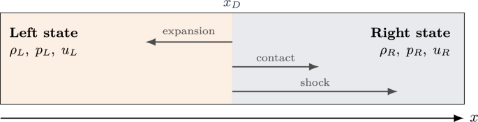
Schematic of a typical planar shock wave problem. \(x_D\) denotes the location of the diaphragm. Rupture of the diaphragm produces an expansion fan (left), a contact surface, and a shock wave (right).
This configuration is a variant of the classical Sod shock tube problem25, which admits an analytic solution consisting of three distinct wave families: a left-going rarefaction fan, a contact discontinuity, and a right-going shock wave.
The numerical solution is computed with the in-house CFD solver Chord26, a structured-grid fourth-order finite volume method. The finite volume method solves the integral form of the compressible Euler equations:
$$\begin{aligned} \frac{d\langle \textbf{U} \rangle _i}{dt} = -\frac{1}{\Delta x} \sum _{d=1}^{D} \left( \langle \vec {F} \rangle _{i + \frac{1}{2}e^d} – \langle \vec {F} \rangle _{i – \frac{1}{2}e^d} \right) \end{aligned}$$
(22)
where the subscript i is a multidimensional cell index, \(\frac{1}{2}e^d\) denotes neighboring face values, and angle brackets denote cell-averaged quantities. Face-averaged fluxes \(\langle \vec {F} \rangle _{i+\frac{1}{2}e^d}\) are computed by reconstructing face-averaged primitive variables W (mass, velocity, pressure) using a fourth-order stencil:
$$\begin{aligned} \langle W \rangle _{i+\frac{1}{2}e^d} = -\frac{1}{12}\langle W \rangle _{i-e^d} + \frac{7}{12}\langle W \rangle _{i} + \frac{7}{12}\langle W \rangle _{i+e^d} – \frac{1}{12}\langle W \rangle _{i+2e^d} + {\mathcal {O}}(\Delta x^4) \end{aligned}$$
(23)
Time integration uses the standard fourth-order Runge–Kutta scheme. In regions of discontinuity, a partial parabolic limiter reduces the stencil order to suppress spurious oscillations. All calculations use double floating-point precision and are written to HDF5 files.
The shock tube dataset comprises 500 simulation cases, each consisting of 43 consecutive timesteps, yielding 21,500 total samples. Cases are generated by varying the left-state pressure \(p_L\) and density \(\rho _L\) while maintaining fixed ratios \(p_L / p_R = 10\) and \(\rho _L / \rho _R = 8\). The pressure takes 20 uniformly spaced values in \(p_L \in [50{,}000,\ 168{,}750]\) Pa with increments of 6,250 Pa, and the density takes 25 uniformly spaced values in \(\rho _L \in [0.5,\ 2.0]\) kg/m\(^3\) with increments of 0.0625 kg/m\(^3\). Each case is advanced with a constant timestep \(\Delta t\) determined by the CFL condition:
$$\begin{aligned} \Delta t = \frac{0.5\,\Delta x}{C} \end{aligned}$$
(24)
where C is the theoretical maximum wave speed. Lower densities and higher left-state pressures correspond to increased sound speed and therefore smaller \(\Delta t\). Across the 500 cases, \(\Delta t\) spans a \(3.7\times\) range from \(3.84 \times 10^{-6}\) s to \(1.41 \times 10^{-5}\) s, with 381 unique values. The timestep \(\Delta t\) is provided to the model as a global conditioning parameter alongside \(p_L\) and \(\rho _L\), enabling G-PARC to adapt its temporal dynamics to each case — a critical distinction from PARCv2, which assumes uniform \(\Delta t\) across all training samples.
The dataset is partitioned as follows (Fig. 7). The training set (400 cases) spans the full range of both \(p_L\) and \(\rho _L\), with all 20 pressure values and all 25 density values represented, providing broad coverage of the parameter space including the full range of \(\Delta t\) values. The validation set (25 cases) is restricted to a narrow band of mid-range pressures (\(p_L \in \{100{,}000,\ 106{,}250\}\) Pa, with one case at 112,500 Pa) paired with densities spanning the full range, evaluating interpolation performance at pressures well-represented during training. The test set (75 cases) is concentrated at the extremes of the parameter space, combining low pressures (\(p_L \in \{50{,}000,\ 56{,}250\}\) Pa) and high pressures (\(p_L \in \{143{,}750,\ 150{,}000,\ 156{,}250,\ 162{,}500,\ 168{,}750\}\) Pa) with extreme densities (\(\rho _L \le 0.8125\) kg/m\(^3\) and \(\rho _L \ge 1.6875\) kg/m\(^3\)). This split deliberately targets the corners of the parameter space, providing a stringent test of extrapolation beyond the densely sampled interior. Notably, the test set includes both the smallest and largest \(\Delta t\) values in the dataset, further challenging the model’s temporal generalization.

Parameter space distribution across the 400 training, 25 validation, and 75 test cases in the \(p_L\)–\(\rho _L\) domain. The split shows that training covers the full interior grid, validation is restricted to a narrow mid-range pressure band, and test cases are deliberately concentrated at the extremes to evaluate out-of-distribution extrapolation.
C: Elastoplastic simulation setup
The elastoplastic dataset is derived from the PLAID benchmark suite using OpenRadioss18. The benchmark, denoted 2D_ElPlDynamics, consists of two-dimensional dynamic nonlinear structural mechanics simulations in large deformation and plane strain regimes, solved with the finite element method. The material is modeled with a nonlinear elastoplastic constitutive law incorporating damage via element erosion, failure, and a non-local regularization method for reducing mesh sensitivity. Each simulation computes the transient deformation of a 2D structure subjected to an imposed displacement on the right boundary and zero displacement on the left boundary18.
Input variability across the dataset arises from the unstructured meshes, which differ in shape, number of nodes, connectivity, and topology. The output fields of interest are the displacement components \(U_x\) and \(U_y\) all defined at the mesh nodes over the simulation horizon.
The full dataset contains 1,000 simulation cases. We randomly partition these into 50 training, 10 validation, and 932 test samples. Prior work utilized 40 A100 GPUs for training on the full dataset. We employ this small-data regime deliberately to evaluate model performance under limited supervision on a single A100-80GB GPU; better results across all models would be expected with access to the full training set.
D: Evaluation metrics
Root Mean Squared Error (RMSE). The RMSE at timestep t measures the average magnitude of prediction error across all N nodes and D variables:
$$\begin{aligned} \textrm{RMSE}(t) = \sqrt{\frac{1}{N} \sum _{i=1}^{N} \left\| \hat{\textbf{y}}_i^t – \textbf{y}_i^t \right\| ^2} \end{aligned}$$
(25)
where \(\hat{\textbf{y}}\) and \(\textbf{y}\) are the predicted and ground truth field values at node i and timestep t, and \(\Vert \cdot \Vert\) denotes the Euclidean norm over D variables.
Relative Root Mean Squared Error (RRMSE). The RRMSE normalizes the RMSE by the root mean square of the ground truth, making it unitless and comparable across variables with different physical scales:
$$\begin{aligned} \textrm{RRMSE}(t) = \frac{\textrm{RMSE}(t)}{\textrm{RMS}(\textbf{y}^t)}, \qquad \textrm{RMS}(\textbf{y}^t) = \sqrt{\frac{1}{N} \sum _{i=1}^{N} \left\| \textbf{y}_i^t \right\| ^2} \end{aligned}$$
(26)
An RRMSE of 0 indicates perfect prediction; values less than 1.0 indicate the model error is smaller than the signal magnitude.
Normalized Mean Squared Error (NMSE). The NMSE normalizes the mean squared error by the variance of the ground truth field, providing a scale-invariant measure of prediction quality.
Structural Similarity Index (SSIM). SSIM measures the similarity between predicted and ground truth fields by jointly evaluating three components: mean field magnitude, field variance, and spatial covariance structure. In physical field prediction, these correspond respectively to whether the model captures the correct overall field level, the correct amplitude of spatial variation, and the correct spatial organization of gradients and features. An SSIM of 1 indicates perfect agreement with the reference field; values approaching 0 indicate poor structural correspondence27.
Nash–Sutcliffe Efficiency (NSE) The Nash–Sutcliffe Efficiency measures predictive skill by comparing the squared prediction error against the variance of the observed water depth field. It is defined as
$$\begin{aligned} \text {NSE} = 1 – \frac{\displaystyle \sum _{i=1}^{N} \left( {\hat{h}}_i – h_i\right) ^2}{\displaystyle \sum _{i=1}^{N} \left( h_i – {\bar{h}}\right) ^2} \end{aligned}$$
(27)
where \({\hat{h}}_i\) and \(h_i\) denote the predicted and reference water depths at node i, N is the total number of nodes, and \({\bar{h}}\) is the mean reference water depth over all nodes. Higher NSE indicates better predictive performance, with \(\text {NSE} = 1\) corresponding to perfect agreement, and values below zero indicating that the prediction is worse than using the mean observed depth as a predictor.
Critical Success Index (CSI) The Critical Success Index evaluates the model’s ability to correctly identify flood exceedance events above a prescribed water-depth threshold. It is defined as
$$\begin{aligned} \text {CSI} = \frac{H_{\text {thr}}}{H_{\text {thr}} + M_{\text {thr}} + FA_{\text {thr}}} \end{aligned}$$
(28)
where \(H_{\text {thr}}\) is the number of hits, \(M_{\text {thr}}\) is the number of misses, and \(FA_{\text {thr}}\) is the number of false alarms for a threshold \(h_{\text {thr}}\). Here, a hit corresponds to a node where both the prediction and the reference solution exceed \(h_{\text {thr}}\), a miss corresponds to a node where only the reference solution exceeds the threshold, and a false alarm corresponds to a node where only the prediction exceeds the threshold. Higher CSI indicates better agreement in identifying significant flood events. Following the fluvial hydrology evaluation protocol, CSI can be reported at thresholds of 0.05 m and 0.30 m to capture both low-magnitude inundation and more operationally significant flooding.
E: Per-variable model predictions
E.1: Fluvial hydrology
See Tables 4,5,6 and Figs. 8,9,10,11.

Top three best performing model for White River Flooding Model Prediction: G-PARC, G-PARC (w/o MLS), MGKAN.

Direct one-shot depth prediction on the Iowa River. Ground-truth and Transolver water-depth fields across the 20-step fluvial rollout. Transolver predicts the entire trajectory in a single forward pass rather than by recurrent integration; at this short horizon its depth field tracks the ground-truth pattern closely, but the output length is fixed at training time and cannot be extended to the longer rollouts reported in the main text.

Direct one-shot depth prediction on the White River. Ground-truth and Transolver water-depth fields across the 20-step fluvial rollout, shown to complement Fig. 9. As above, Transolver produces all timesteps in one pass and is accurate over the fixed 20-step horizon, the maximum its output head supports.

Worst two baseline models for Iowa River Flooding Model Prediction: MGNET and GraphSAGE.
E.2: Planar shock wave
See Tables 7,8 and Figs. 12,13,14,15,16.

Planar Shockwave Model Prediction for PARCv2. PARCv2 predicts the total energy E (J/m\(^3\)), which represents the sum of internal and kinetic energy per unit volume. PARCv2 fails to produce a meaningful prediction.

Predicted density fields for the top three models (G-PARC, G-PARC (w/o MLS), and MGKAN) on the same representative test case as Figure 3.

Predicted total energy fields for the top three models (G-PARC, G-PARC (w/o MLS), and MGKAN) on the same representative test case as Figure 3.

Predicted x-momentum fields for the two worst-performing models (MGNET and GraphSAGE) on the same representative test case as Figure 3, illustrating catastrophic rollout failure under long-horizon autoregressive prediction.

Direct one-shot x-momentum prediction on a shock-tube Riemann problem. Ground-truth, G-PARC, and Transolver x-momentum (\(\rho u_x\)) fields for the compressible-Euler shock tube with left-state initial conditions \(p_L = 143{,}750\), \(\rho _L = 0.5625\). Transolver produces visual artifacts across the domain.
E.3: Elastoplastic
See Figs. 17,18 and Tables 9,10.

Worst two performing models for elastoplastic dataset: MGNET and GraphSAGE. Both models fail to predict meaningful results.

Direct one-shot displacement prediction on an elastoplastic impact simulation. Ground-truth, G-PARC, and Transolver displacement-magnitude fields for elastoplastic test simulation 179. Transolver predicts the entire trajectory in a single forward pass rather than by recurrent integration; on this domain it attains the lower pooled RRMSE reported in Table 1.