Evolutionarily conserved short linear motifs drive actin filament binding

Pipeline overview

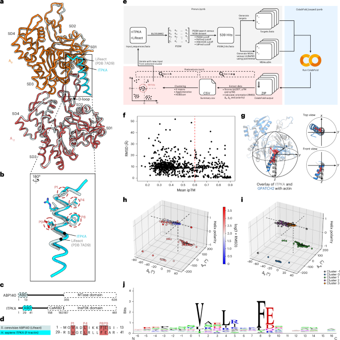
The SLiMFold pipeline, which integrates multiple bioinformatic tools to systematically identify, filter and validate candidate motifs was used for the identification of actin filament-binding SLiMs. Among others, the SLiMFold pipeline integrates ColabFold⁴⁵, which utilizes AlphaFold2 Multimer to predict the structures of identified actin-binding candidates. To increase the specificity and accuracy of the pipeline, actin filament-binding SLiMs were identified by running three iterations, each involving the followings steps.

Prerun

The process begins with Prerun.ipynb, where hypothesized SLiMs (in this study, the aligned sequences of ITPKA and Lifeact ABDs from P1 to P9) were used along with the BLOSUM62 substitution matrix¹⁰⁷ to create a PSSM. This PSSM was used to scan the human proteome (NCBI Taxonomy ID: 9606) for putative motif hits. To further filter out false positives, we incorporated the following criteria.

• PSSM score: The matrix was used to score sequences in the database, identifying motifs similar to the hypothesized SLiMs¹⁰⁸.

• IUPRED: Predicts intrinsically disordered regions, highlighting regions suitable for motif embedding. The mean IUPRED score was calculated for the motif and its 60-residue flanking regions (N- and C-terminal)⁴³.

• ANCHOR: Identifies regions in intrinsically disordered regions that are likely to bind structured partners. The mean ANCHOR value was calculated within the motif⁴².

• PSIPRED: Predicts the probability of secondary structures (helix, β-strand and random coil)⁴¹.

All cutoffs for these criteria were progressively relaxed across iterations (described in the next paragraph). This approach allowed the identification of additional hits while iteratively strengthening the PSSM, reducing false positives. Each hit was extended by ±20 flanking residues for subsequent homology searches and redundant sequences were removed. Each hit was then paired with the bait sequence (the human actin sequence) and saved as a separate FASTA file, formatted for direct compatibility with ColabFold.

For each hit, MSAs were generated using jackhmmer⁴⁴ with the UniRef90 database. The following jackhmmer parameters were applied: five iterations; e-value = 1 × 10⁻⁵; no f1 or f2 filter (original AlphaFold2 code: one iteration; e-value = 1 × 10⁻⁵; f1, 0.0005; f2, 0.00005). The modified jackhmmer parameters improved the number of sequences retrieved, probably enhancing detection of more distant homologues. In addition, parallelization was implemented to process multiple hits simultaneously, significantly speeding up the alignment step. The sto-file for the bait sequence was constructed in the same manner. Output alignments were reformatted to A3M format using the reformat.pl script in HH-suite¹⁰⁹ to ensure compatibility with downstream structure prediction tools. Alignments were sorted and combined to meet AlphaFold2 Multimer input criteria.

ColabFold looped

The ColabFold_looped.ipynb notebook, originally developed by the Steinegger laboratory⁴⁵, was modified to enable batch processing and the integration of custom MSAs, making it more suitable for the SLiMFold workflow. These modifications were designed to streamline the process and enhance flexibility when handling multiple input sequences. In the modified version, the notebook was adapted to loop through all FASTA files in a specified folder, such as one located in Google Drive. This automation allowed for seamless processing of multiple sequences without the need for manual input, significantly improving the workflow efficiency. In addition, the modified notebook incorporated the ability to retrieve precomputed A3M files from another designated folder. These alignments, created during the Prerun.ipynb step, were matched to their corresponding FASTA files based on their names. This ensured accurate integration of the custom MSAs into the ColabFold predictions. To manage outputs effectively, the notebook allowed users to specify a folder for storing results. This organizational set-up made it easier to handle and analyse the results of large-scale computations.

Compared with the original ColabFold batch notebook, these modifications introduced enhanced flexibility by supporting custom MSAs and allowing adjustments to the number of seeds used in the AlphaFold2 Multimer predictions.

Post analysis

The post-analysis step was performed using the Postanalysis.ipynb script, which systematically processed and analysed the outputs from the SLiMFold pipeline. This step integrated sequence and structural data to evaluate the conformational and functional relevance of candidate actin filament-binding SLiMs. The pLDDT, pTM and ipTM scores were extracted to assess prediction confidence and interaction reliability of each predicted structure. Structures with ipTM scores below 0.6 were excluded from further analysis, ensuring a focus on high-confidence predictions. Each remaining structure was aligned to a reference PDB file (in this study, the ITPKA–actin complex, PDB: 9QGK) to evaluate conformational similarity.

The RMSD between the alpha carbon (Cα) atoms of the predicted structure and the reference structure at the motif positions (P1 to P9) was calculated to quantify structural similarity. RMSD was computed as:

where N is the number of aligned residues, \({x}_{i}\) represents the atomic coordinates of a residue in the predicted structure and \({x}_{{\rm{ref}}}\) represents the corresponding coordinates in the reference structure.

Angular analysis was performed using vector-based calculations, where the spatial coordinates of the alpha carbon (Cα) atoms of key residues in the SLiM (P1 to P9) were used to define vectors representing the orientation of the motif. Two angles, \(\varphi\) (azimuthal angle in the x–y plane) and \(\theta\) (polar angle relative to the z axis), were calculated to quantify the orientation of the motif relative to the reference vector:

where \(x\) and \(y\) are the coordinates of the vector projection in the x–y plane, \(z\) is the zcoordinate of the vector and |\(v\)| is the magnitude of the vector. Helix polarity was also calculated to capture the directionality of the structural alignment of the predicted motif. The Δφ and Δθ values, representing the differences between the angles of the predicted and reference structures, were calculated for each candidate SLiM. These metrics, along with RMSD and polarity, provided a comprehensive structural profile for clustering.

Clustering was performed using the hdbscan⁴⁶ algorithm, leveraging RMSD, Δφ, Δθ and polarity as input features. The clustering parameters, including minimum cluster size and minimum samples, were optimized using the following metrics.

• Silhouette score: Evaluates cluster separation and cohesion.

• Davies–Bouldin index: Measures intra-cluster similarity relative to inter-cluster separation.

• Calinski–Harabasz index: Assesses the ratio of between-cluster dispersion to within-cluster dispersion.

Optimal clustering parameters were selected based on these indices, ensuring robust and meaningful grouping of structurally similar SLiMs. For further analysis, all structures belonging to a single cluster were exported as a PyMOL session file (.pml), enabling manual inspection and visualization. For each cluster, the corresponding sequences were compiled into a FASTA file. These sequences were used to generate sequence logos¹¹⁰, highlighting conserved residues and identifying potential functional motifs. In addition, each sequence was mapped to its corresponding gene using the NCBI database. This mapping facilitated gene ontology (GO) enrichment analysis, allowing functional insights into the biological roles of the identified SLiMs.

Cloning strategies

All constructs were generated via PCR-based cloning using high-fidelity polymerases (Q5 or Phusion; M0491S or M0530S, New England Biolabs Inc.) following the manufacturer’s instructions. For inserting longer DNA fragments such as full-length protein sequences, we employed T4 sequence and ligation independent cloning¹¹¹ (T4 DNA Polymerase; M0203S, New England Biolabs Inc.), which relies on overlaps of about 30 nucleotides between the vector and insert for seamless assembly. Short peptides or specific mutations were introduced using a ‘QuickChange-like’ site-directed mutagenesis protocol, wherein primer pairs incorporated short (8–12 nucleotides) overlaps at their 5′ ends; the PCR products were subsequently treated with DpnI (R0176S, New England Biolabs Inc.) to remove the template and then transformed into Escherichia coli XL1-Blue (200249, Agilent Technologies, Inc.). Alternatively, the PCR products were processed using a kinase–ligase–DpnI enzyme mix (M0554S, New England Biolabs Inc.) to remove the template and ligate the new amplicon. For bacterial expression, PCR products were cloned into pSF421-based expression vectors (for example, pSF421_10xHis_GFP_TEV); for eukaryotic expression in mammalian cells (for example, H1299), target genes were inserted into an mEGFP-N1 backbone. All final plasmids were verified by Sanger sequencing (Microsynth Seqlab GmbH). Verified constructs were subsequently transformed into E. coli Rosetta (DE3) cells (Novagen, Merck KGaA) for bacterial protein expression or transfected into mammalian cells. Complete plasmid lists, vector maps, sequencing results and primer sequences are provided in Supplementary Tables 5,6 and Source data. The oligonucleotides used in this study were designed in-house and synthesised by Integrated DNA Technologies (IDT).

Actin purification

Actin was prepared from Gallus gallus (chicken) skeletal muscle as described¹¹². The final purification step was performed using a HiLoad 16/600 Superdex 200 column equilibrated with globular actin buffer (5 mM Tris–HCl pH 7.5, 0.2 mM CaCl₂, 0.5 mM dithiothreitol and 0.2 mM ATP).

Expression and purification of ITPKA and GFP peptides

All constructs were expressed in E. coli Rosetta (DE3) competent cells (Novagen, Merck KGaA). The cells were cultured in Terrific Broth at 37 °C to an optical density at 600 nm of 0.6–1.0. Protein expression was induced with 0.2 mM isopropyl β-D-1-thiogalactopyranoside and incubation at 18 °C for 16 h for ITPKA or at 37 °C for 4 h for the GFP-tagged peptides. After induction, the cells were harvested by centrifugation at 3,000g and 4 °C for 20 min. The cell pellets were resuspended in cold PBS buffer, centrifuged at 2,000g and 4 °C for 30 min, flash-frozen in liquid nitrogen and stored at −80 °C.

For protein purification, the cell pellets were resuspended in ice-cold Buffer A (50 mM Tris–HCl pH 7.4, 400 mM NaCl, 3 mM MgCl₂ and 1 mM β-mercaptoethanol for ITPKA; 50 mM Tris–HCl pH 7.4, 300 mM NaCl and 1 mM β-mercaptoethanol for GFP peptides) and homogenized using an IKA ULTRA-TURRAX disperser (IKA-Werke GmbH & Co.). DNase I was added and the cells were lysed with a Constant Cell Disruption System (Constant Systems Limited) at 1.8 kbar. Following lysis, phenylmethylsulfonyl fluoride (final concentration of 1 mM) and imidazole (final concentration of 25 mM) were added to the cells. The cell debris was removed by centrifugation at 43,000g and 4 °C for 30 min, and the supernatant was incubated with Ni-NTA agarose resin (SERVA Electrophoresis GmbH) for 30 min at 4 °C. The bound proteins were eluted using a gradient of Buffer B (Buffer A with 500 mM imidazole). Fractions were analysed by SDS–PAGE, and those with >90% purity were pooled and then dialysed overnight at 4 °C in Buffer A.

Subsequently, the dialysed proteins (GFP peptides) were concentrated to 0.5–2 ml using Amicon Ultra Centrifugal Filters (Merck-Millipore) and further purified by size-exclusion chromatography using a HiLoad Superdex 16/600 200 pg Gel Filtration Column (Cytiva) on an NGC liquid chromatography system (Bio-Rad Laboratories) equilibrated with Buffer D (50 mM Tris–HCl pH 7.4, 150 mM NaCl, 3 mM MgCl₂ and 1 mM β-mercaptoethanol for ITPKA; 50 mM Tris–HCl pH 7.4, 150 mM NaCl and 1 mM β-mercaptoethanol for GFP peptides). The peak fractions were concentrated, aliquoted and then flash-frozen in liquid nitrogen, and stored at −80 °C.

Acquisition and processing of cryogenic electron microscopy data

We initiated all sample preparations using frozen aliquots of globular actin. To convert globular actin into filamentous actin, the samples were first thawed, followed by centrifugation at 100,000g for 30 min to eliminate potential aggregates. The polymerization process involved the addition of F buffer (20 mM Tris-HCl pH 7.5, 100 mM KCl, 2 mM MgCl₂, 0.5 mM ATP, 1 mM EGTA, 1 mM dithiothreitol), followed by incubation at room temperature for 1 h. Subsequently, we collected the filaments by centrifugation at 100,000g and 4 °C for 1 h, and resuspended them in F buffer supplemented with phalloidin at twice the molar concentration of the actin filaments.

Quantifoil 200-mesh 2.0/1.0 holey carbon grids were used for cryo-EM grid preparation. Specifically, for phalloidin-stabilized actin filaments, we applied 3.5 μl of 1 μM solution onto glow-discharged grids. For the phalloidin-stabilized actin filament–ITPKA complex, we initially applied 2 μl of 1 μM phalloidin-stabilized actin filaments to the grids. Subsequently, we added 2 μl of 10 μM ITPKA and mixed it directly on the grids immediately before plunge-freezing in a liquid ethane–propane mixture using a Vitrobot Mark IV system (FEI). Datasets were collected on an FEI Titan Krios transmission electron microscope (300 kV; Gatan K3 camera; pixel size, 0.826 Å; dose per frame, 1.4; defocus range, 0.8–3.0 μm).

Single-particle helical reconstruction was performed using Relion 4 (ref. ¹¹³). Videos were first motion-corrected using MotionCor2 (ref. ¹¹⁴) and then the contrast transfer function estimation was performed using CTFFIND4 (ref. ¹¹⁵). Particle segments picking model was trained in cryolo 1.7 (ref. ¹¹⁶). The helical segments were extracted into 360 × 360 boxes and the junk segments were excluded after two-dimensional classification. The initial helical parameters of a helical rise of 27.3 Å and a helical twist of −166.5° were applied for three-dimensional classification and autorefinement in Relion 4.0. Overall, gold-standard resolution (Fourier shell correlation = 0.143) was calculated in Relion 4.0. The statistics for data collection and processing are listed in Supplementary Table 2.

For the actin filament–USP54 M1 complex, actin filaments were prepared without phalloidin. A total of 2 μl of 4.75 μM actin filaments were applied to glow-discharged grids, followed by 2 μl of 105.83 μM USP54 M1–EGFP fusion protein. The components were mixed directly on the grids immediately before plunge-freezing in liquid ethane using a Vitrobot Mark IV. Data were collected on a Glacios transmission electron microscope operated at 200 kV and equipped with a Falcon 4i camera, an energy filter with a 10 eV slit width and a 50 μm C2 aperture. Images were recorded at a calibrated pixel size of 0.91 Å, with a total accumulated dose of 40 e⁻ Å⁻² and a defocus range of –0.5 to –2.0 μm. Motion correction, contrast transfer function estimation, particle picking, two-dimensional classification and helical refinement were performed in CryoSPARC^{117,118,119,120,121}. Helical segments were identified using the Filament Tracer tool, and non-specific particles were removed by two-dimensional classification. The remaining segments were further refined through heterogeneous classification, with the best three-dimensional class subjected to final helical refinement. The resolution of the reconstruction was determined by gold-standard Fourier shell correlation at the 0.143 criterion. A summary of this data collection and image processing statistics is provided in Supplementary Table 2.

Model building and refinement

Previously published models of phalloidin-bound actin filaments (PDB: 6T20, ref. ¹²²; 7BTI ref. ⁴⁰) and the AlphaFold2 structure of ITPKA and USP54 M1 SFM were used as initial models. Models were initially built in ChimeraX 1.7 (ref. ¹²³), and further refined against the cryo-EM maps using ISOLDE¹²⁴ and real space refinement in Phenix¹²⁵. The detailed model information and validation statistics for final models are described in Supplementary Table 2.

Cell culture

NCI-H1299 (H1299) cells were provided by C. Günes (Hamburg, Germany). For detailed cellular characteristics, refer to the American Type Culture Collection. Cell line authentication was performed by the Leibniz Institute DSMZ–German Collection of Microorganisms and Cell Cultures (28 January 2025) using analysis of 17 short-tandem-repeat loci. The cells were cultured in Dulbecco’s modified eagle’s medium supplemented with 10% (vol/vol) fetal calf serum, 4 mM L-glutamine, 100 μg ml⁻¹ streptomycin and 100 U ml⁻¹ penicillin. The culturing conditions were rigorously maintained to ensure optimal growth and viability. In addition, the cells were tested regularly for mycoplasma contamination to ensure the experiments were conducted with mycoplasma-free cells.

Primary human monocytes were isolated from buffy coats (provided by F. Bentzien, Transfusion Medicine, UKE, Hamburg, Germany). A 20 ml volume of blood was coated on 15 ml lymphocyte separation medium 1077 (PromoCell) and centrifuged at 4 °C and 460gfor 30 min. The buffy coats were transferred to a new 50 ml Falcon tube and made up to 50 ml with cold RPMI (Gibco). Leukocyte fractions were washed twice in RPMI and centrifuged for 10 min, as described earlier. Enriched leukocytes were resuspended in 400 μl monocyte buffer (5 mM EDTA and 0.5% human serum albumin in Dulbecco’s PBS, pH 7.4), mixed with 100 μl of magnetic beads suspension coupled to antibodies to CD14 (Miltenyi Biotec) and incubated on ice for 15 min. The mixture was subsequently loaded onto Separation columns LS (Miltenyi Biotec) that had been previously placed in a magnetic holder and equilibrated with 500 μl cold monocyte buffer. CD14⁺ monocytes trapped in the column were washed with 500 μl monocyte buffer and then eluted with 1 ml monocyte buffer into 15 ml cold RPMI after removal from the magnets. After centrifugation at 460gand 4 °C for 10 min, the supernatant was removed, and the cells were resuspended in 40 ml RPMI and seeded on a six-well plate (Sarstedt) at a density of 2 × 10⁶ cells per well. The monocytes were allowed to adhere for 1 h, after which the RPMI medium was replaced with 2 ml monocyte culture medium (RPMI substituted with 20% human serum and 1% penicillin–streptomycin; Sigma-Aldrich). The monocytes were cultured in an incubator at 37 °C, 5% CO₂ and 90% humidity. Isolated monocytes were differentiated for at least six days.

Transfection of cells

For the H1299 cells, a total of 2.5 × 10⁴ cells were seeded into eight-well chamber slides (Ibidi) and incubated for 16 h. The cells were then transfected with 0.5 µg of any mEGFP-N1-Peptide or mEGFP-N1-FL-Proteins using K2 transfection reagent (T060-0.75, Biontex Laboratories GmbH) according to the manufacturer’s instructions. After 24 h, the cells were fixed with 4% paraformaldehyde in 4% sucrose, stained with rhodamine-conjugated phalloidin (ab235138, Abcam Limited) and analysed by fluorescence microscopy using an Olympus IXplore Live microscope imaging system and FV3000 confocal laser-scanning microscope.

Macrophages were detached by incubation with accutase (Invitrogen) for at least 30 min in culturing conditions. The cells were collected with monocyte culture medium, washed in PBS pH 7.3 and resuspended in R Buffer (at a concentration of 1 × 10⁶ cells per 100 µl buffer, 10 µg DNA), provided by the Neon Transfection System (Invitrogen). The macrophages were transiently transfected with plasmid DNA with the following settings: voltage, 1,000 V; width, 40 ms; two pulses. The transfected cells were resuspended in RPMI and seeded on 12-mm glass coverslips (1 × 10⁵ cells per coverslip). The cells were left to adhere for 1 h under culturing conditions. Thereafter, 1 ml of monocyte culture medium was added to the cells, followed by overnight incubation.

Immunofluorescence and microscopy

Cells were fixed in PBS containing 3.7% formaldehyde for 10 min, followed by permeabilization in PBS containing 0.5% Triton X-100 for 10 min. Thereafter, the cells were incubated for 60 min in blocking solution (2% BSA in PBS) with 1:400 phalloidin-568. The cells were washed three times in PBS and mounted on glass slides with FluoromountG (Invitrogen) containing 4′,6-diamidino-2-phenylindole (Sigma-Aldrich). Images of fixed samples were acquired using an Olympus FV3000 equipped confocal laser-scanning microscope with an ×60 UPlanApo HR oil objective and the Olympus FV3000 software.

Poji macro analysis

Localization of peptides to actin filaments at podosomes was evaluated using Poji¹²⁶. The Poji macro is a semi-automated ImageJ/Fiji plugin created to characterize protein distribution and enrichment at podosomes. Profile analysis begins with the processing of raw microscopy data as separate fluorescence channels, with the actin filament channel, defined by phalloidin-568 staining, as a reference. To enable good detection quality at the ventral surface of transfected cells, prominence was set to 100 pixels and the detection size of the podosomal circular region of interest (ROI) to 25 pixels. These parameters were kept through all the experiments and cells analysed. At least three cells were analysed simultaneously to reduce the workload. During analysis, fluorescence intensities of 360° intensity profiles of single podosomal ROIs were measured.

Poji generates a circular ROI around each analysed podosome, with subsequent stacking of individual podosomal ROIs to create average intensity profiles and rotational line scans. The Poji radial profiles at optical z plane of highest actin filament intensity, with mean ± s.d. values of the fluorescence intensity of actin filament and the respective SFM peptides, were determined for n ≥ 3 cells, with 240 podosomes per transfected peptide.

Co-sedimentation assay and apparent K
_d determination

The K_d,appand binding strength of the interaction between the ABP and filamentous actin were determined using an actin filament co-sedimentation assay.

For this, preparations were made using frozen aliquots of globular actin. To convert globular actin into actin filaments, the samples were thawed and centrifuged at 100,000g for 30 min to eliminate potential aggregates. For actin polymerization, F buffer (see above) was added and the samples were then incubated at room temperature for 1 h. The resulting actin filaments were mixed with 4 µM EGFP–SFM peptide and incubated for 1 h at room temperature before co-sedimentation at 100,000g for 30 min. Thereafter, the pellet was resuspended in sample buffer, heated to 95 °C for 15 min and analysed by western blotting employing an antibody to EGFP. We then plotted densitometry (D) as a function of the total actin concentration \({[{\rm{actin}}]}_{{\rm{total}}}\). These data were fit in GraphPad Prism using the ‘One-site specific binding’ hyperbolic model:

All experiments were performed in triplicate to ensure reproducibility. EGFP–SFM peptide (fixed concentration of 4 µM) was incubated with Varying concentrations of actin (0–200 µM). In each replicate, a negative control (0 µM actin) verified background signal.

For the binding strength determination of USP54 and SHROOM3 mutants (M1, M2, M3 and M4), the proteins were employed at a final concentration of 4 µM and actin filaments at 12 µM. Densitometric analysis was performed on the western blot results, quantifying the signal intensity of the bound EGFP–SFM peptide in the pellet fraction to assess differences in binding strength among the mutants. The densitometry values were corrected by subtraction of the negative control (SFM with 0 µM actin).

As a specificity control, EGFP alone as well as the Lifeact P1/P8 constructs were used (Extended Data Fig. 6).

SDS–PAGE and western blotting

Equal volumes of samples were loaded onto 12% polyacrylamide gels for SDS–PAGE. Electrophoresis was performed at 120 V until the dye front reached the bottom of the gel. The separated proteins were transferred onto nitrocellulose membranes using a wet transfer system at 60 V for 90 min in 1×blot buffer. Non-specific binding was blocked by incubating the membranes in 5% (wt/vol) non-fat dry milk in Tris-buffered saline with Tween 20 (TBST) for 1 h at room temperature. The membranes were incubated overnight at 4 °C with the primary antibody specific to EGFP (mouse anti-EGFP, 1:1,1000; catalogue number 11814460001, Roche Applied Science) diluted in blocking buffer. After three washes with TBST, the membranes were incubated with secondary antibody for EGFP detection (goat anti-mouse; 1:10,000 dilution in TBST) at room temperature for 1 h. Protein bands were detected using a chemiluminescence reagent (Cytiva Amersham ECL prime western blot detection reagent) and imaged using an INTAS ECL chemocam system (INTAS Science Imaging Instruments GmbH). Band intensities were analysed using ImageJ¹²⁷ with consistent ROIs applied across all lanes and local background subtraction performed individually. Linearity of the detection range was verified using a calibration curve to ensure the measurements remained within the dynamic range of the assay. Western blot detection was chosen instead of Coomassie staining to enable sensitive detection of EGFP–SFM peptides. The K_d,app values are therefore comparable within this experimental series but should not be directly compared with values obtained using alternative detection methods.

Position-specific frequency matrix

We developed a pipeline for generating PSFMs that quantify amino acid conservation at each position across a set of sequences, focusing specifically on peptides with high affinity or strong co-localization. Multiple sequence alignments derived from SLiMFold’s jackhmmer output were manually curated to remove alignments with names indicating different proteins, ensuring retention of only true homologues. These curated MSAs served as input for generating individual frequency tables for each peptide, which were then averaged to account for variations in the number of homologous sequences. A 23 × Nmatrix (where N is the sequence length) was generated, with each element representing the proportion of a specific amino acid at a given position. To reduce skewness in the data and emphasise subtle conservation trends, a square root transformation was applied to the matrix. Heat maps of the PSFMs were visualized using matplotlib, with conserved positions annotated and residue indices labelled for interpretation. Detailed code has been provided¹²⁸.

Phylogenetic and motif analysis

We conducted a comprehensive phylogenetic analysis to investigate the evolutionary history of proteins containing actin-filament-binding motifs and their isoforms. Orthologous sequences were retrieved from OrthoDB¹²⁹ and aligned using DECIPHER¹³⁰ (100 iterations, 200 refinements). Maximum likelihood phylogenetic trees were constructed using IQ-TREE 2 (WAG + G model; 1,000 ultrafast bootstraps)¹³¹. Isoform sequences were identified and filtered based on header annotations and their phylogenetic clustering was visualized. Taxonomic information was incorporated to determine the MRCA of isoform clusters. Actin filament-binding motifs were extracted using regular expressions and filtered based on predicted disorder (IUPRED)⁴³, anchor regions (ANCHOR)⁴² and random coil propensity (PSIPRED)⁴¹. Position-specific scoring matrices were generated and iteratively used to refine motif identification. The MRCA of motif-containing sequences was determined using isoform-specific trees. Motif distribution was validated by mapping motifs to a taxon-based tree. Motif development across isoforms and taxonomic classes was analysed using frequency matrices. Sequence logos¹¹⁰ were generated from PSSMs. For nucleotide-level analyses, the corresponding DNA sequences were retrieved from NCBI, filtered for ambiguous bases and stop codons, and codon-aligned using PRANK¹³². Phylogenetic trees were inferred with IQ-TREE 2 (GTR + G model)¹³¹, and dN/dS analysis was performed using HyPhy¹³³. Detailed code and parameter settings are provided (Source data).

Molecular dynamics simulation and actin-filament persistence length calculation

The MD simulations were performed with GROMACS2022.4 (ref. ^{134,135,136,137}) using the CHARMM36m protein force field^138,139. Starting coordinates were derived from the corresponding cryo-EM structures to ensure the most-accurate representation of each peptide–protein interface. Therefore, the asymmetric unit of the fitted cryo-EM models was expanded into a 13-subunit filament using a filament screw transformation in UCSF ChimeraX¹⁴⁰. Specifically, the actin–ITPKA and actin–USP54 M1 systems were initiated from their corresponding experimental reconstructions. To provide a rigorous baseline, the actin-only control was generated by computationally removing the peptide from the ITPKA-bound scaffold. Although the initial coordinates for each SFM-bound system reflect their specific experimental binding modes, the subsequent all-atom MD simulations at 310 K allow all systems to explore thermally accessible conformations.

All expanded actin filaments were simulated in an ADP:Mg²⁺ bound state using the same protocol. Briefly, actin filaments were solvated in a cubic box with periodic boundary conditions and an initial minimum distance of 2 nm to all boundaries. All systems were charge-neutralized by the addition of potassium ions; a total KCl concentration of 0.18 M was used to approximate cytosolic salt concentrations. To broadly relax the systems, steepest-descent energy minimization was conducted, resulting in convergence to machine precision within 4,000–5,000 steps. Equilibration of temperature and pressure was achieved by two consecutive 100-ps equilibration MD runs. Temperature equilibration was performed in the NVT ensemble with stochastic velocity rescaling using the V-rescale thermostat¹⁴¹ at 310 K and a time constant of 0.1 ps. Separate temperature coupling groups were applied for the solute and the solvent. Subsequently, pressure coupling was achieved in the NPT ensemble by isotropic scaling of box vectors with the C-rescale barostat¹⁴² at 1 bar and a time constant of 2.0 ps (compressibility of 4.5 × 10⁻⁵ bar⁻¹). All equilibration runs involved a position restraint potential with a force constant of 1,000 kJ mol⁻¹ nm⁻² for solute atoms including actin, peptide chains, ADP and Mg²⁺ ions.

Molecular dynamics production runs were conducted with the leap-frog integrator using a time step of 2 fs and coordinates were saved every 25 ps. While the same temperature coupling scheme as applied in the equilibration runs was used, isotropic pressure coupling was performed with the Parrinello–Rahman barostat¹⁴³ at 1 bar with a time constant of 2 ps (compressibility of 4.5 × 10⁻⁵ bar⁻¹). Hydrogen bond constraints were implemented with the Linear Constraint Solver using an order of four and one iteration¹⁴⁴. Non-bonded interactions were treated with the Verlet cutoff scheme with grid-based neighbour searching. Neighbour lists were updated every 20 steps (40 fs) using a cutoff of 12 Å. Short-range van der Waals interactions were truncated at 12 Å by force-switching between 10 and 12 Å. Long-range electrostatics were calculated using the particle mesh Ewald method^145,146 with a cutoff of 12 Å as well as fourth-order interpolation and 1.6 Å grid spacing for the fast Fourier transform grid. No dispersion correction was used with the CHARMM36m protein force field.

All trajectory analyses were performed using MDAnalysis^147,148 in Python. Before analysis, MD trajectories were pre-processed with GROMACS tools to fix broken molecules and remove periodic boundary conditions as well as rotation and translation. For structural analyses (RMSD, RMSF and contacts), water and potassium ions were removed. To ensure analysis of equilibrated systems, the first 4 ns of each trajectory were discarded and subsequent analyses were performed on the 4–40 ns time window.

To calculate the L_p of actin filaments, pre-processed trajectories were read with MDAnalysis and a filament centreline was built by computing actin monomer centreline points based on the per-frame centre of mass (COM) of all atoms for each actin monomer¹⁴⁹.

Discrete tangents are then computed from centerline point differences:

Removal of spontaneous curvature was achieved by rotating \({{\boldsymbol{\tau }}}_{{\boldsymbol{i}}}\) such that the frame-averaged tangent aligns with the z axis. Finally, tangent–tangent correlations were computed as:

By fitting the first three monotonically decreasing points of \(\mathrm{ln}\left\langle \cos \theta \left(s\right)\right\rangle\) versus \(s\) (with \(s=k\delta s\)), the L_p can be determined:

The global RMSD was computed for Cα atoms relative to the initial frame using the MDAnalysis RMSD module. To avoid edge effects from filament termini, only interior actin chains (chains 2–10 of the 13-mer, chain index starting from zero) were included in the analysis. Per-chain RMSD trajectories were computed independently and aggregated to yield mean ± s.d. values across the filament. The RMSF of each residue was calculated using all heavy atoms excluding solvent and potassium ions with MDAnalysis. For each interior chain, per-residue RMSF values were computed after alignment to the mean structure. The values were then averaged across chains to generate mean ± s.d. profiles along the actin sequence (residues 1–375). Differential RMSF (ΔRMSF) was calculated by subtracting the actin-alone RMSF profile from each SFM-bound condition.

Atomic contacts between SFM peptides (ITPKA or USP54 M1) and actin were quantified using a distance cutoff of 4.0 Å applied to sidechain heavy atoms. For each SFM peptide chain (11 of 13 copies per filament considered), contacts with neighbouring actin subunits were evaluated at each trajectory frame. A residue–residue contact was defined as present when any heavy-atom pair fell within the cutoff distance. Contact frequency matrices were computed as the fraction of frames (normalized to the total number of frames × the number of SFM chains in contact) in which each SFM–actin residue pair was in contact. Time-resolved contact occupancy for individual SFM residues was calculated as the fraction of SFM peptides in contact with any actin residue at each time point. Actin contact occupancy profiles were computed as the fraction of trajectory frames in which each actin residue contacted at least one atom from any SFM peptide, aggregated across all SFM chains.

To monitor actin inter-subunit contacts, specific residue pairs were tracked over the trajectory. For inter-chain contacts (chain N with chain N−2), sidechain heavy atoms were selected and contacts were defined using a distance cutoff of 4.0 Å. Binary contact occurrence (present/absent) was recorded for each chain pair in each frame and the results were aggregated across all valid chain pairs in the interior of the filament. Time-resolved contact density was computed by binning the trajectory into 200-ps windows and calculating the fraction of chain pairs exhibiting the contact within each bin.

To visualize D-loop conformational heterogeneity, trajectory snapshots were extracted at regular intervals (first 4 ns discarded, snapshot every 1.8 ns from the remaining 36 ns) and superimposed. The D-loop coordinates (residues 35–55) from all frames were then overlaid to generate conformational ensembles for each condition. Representative structures were rendered in PyMOL¹⁴⁹ to qualitatively assess the extent of conformational sampling in each system.

To analyse time-dependent conformational fluctuations of filament-internal actin protomers, the dihedral angle defined by the actin subdomains SD2-SD1-SD3-SD4 was computed as follows. The actin subdomain definition was adapted from Iyer and colleagues¹⁵⁰: SD1 residues 1–32, 70–144, 338–375; SD2 residues 33–69; SD3 residues 145–180 and 270–337; SD4 residues 181–269. Due to previously described edge effects in protomers located at the pointed or barbed end of the actin filament, the two terminal actin protomers located at each of the filament ends were excluded from the analysis (13-mer filament with nine internal actin protomers). For each internal protomer, the COM of Cα atoms belonging to each subdomain was calculated. The dihedral angle was then determined from the four COM points (SD2-SD1-SD3-SD4) for every trajectory frame. To obtain a filament-averaged dihedral angle for each frame, the individual dihedral angles of all nine internal actin protomers were averaged. For visualization of time-dependent dihedral angle changes, circular running means were calculated with a window size of 2 ns.

Gene ontology enrichment analysis

To elucidate the biological functions and cellular components associated with SFM-containing proteins, we performed GO enrichment analysis using ShinyGO¹⁵¹. The analysis aimed to identify over-represented GO terms within three primary categories: biological process, cellular component and molecular function. We compiled a comprehensive list of SFM-containing proteins identified in this study as the query set. Utilizing ShinyGO with its standard parameters, we input the query set to perform the enrichment analysis. The analysis employed the default settings for multiple-testing correction, including the false-discovery rate, ensuring that only GO terms with an adjusted P value of <0.05 were considered significantly enriched.

AlphaMissense

For each of the 12 proteins examined in this study, the AlphaMissense pathogenicity score¹⁵² was retrieved using the canonical UniProt ID. The relevant amino acid positions were then manually aligned based on the SFM coordinates. Residues flanking the motif (positions −30 to −20 and +30 to +40) served as control values for comparative analysis. After extracting the AlphaMissense scores for all 12 proteins, the mean score at each aligned position was calculated and the s.e.m. determined. Statistical evaluation of differences between motif residues and the flanking control positions was performed via one-way analysis of variance with multiple comparisons.

Phosphorylation prediction

All SFM-containing protein sequences used in this study were analysed with NetPhos 3.1 (ref. ¹⁵³). For each sequence position containing Ser or Thr, a site-level maximum score across all NetPhos kinase models was computed. Motif-relative positional groups were defined a priori as N-edge (P−2 to P0), C-edge (P10 to P12), in-ring interacting (P1, P4, P5, P8 and P9), in-ring non-interacting (P2, P3, P6 and P7) and outside (all remaining positions). For each group, unique sequence, position (S/T) sites and the subset with high-confidence predictions (score ≥ 0.90) were counted, with outside serving as background. Enrichment of high-confidence sites relative to outside was quantified as odds ratios with Wald 95% confidence intervals; when necessary, a Haldane–Anscombe correction (0.5 added to each cell) was applied. Significance was assessed using two-sided Fisher’s exact tests. Results were visualized as bar charts of high-confidence fractions, forest plots of odds ratio ± 95% confidence intervals and kinase-resolved position plots.

Statistics and reproducibility

The Poji macro is a semi-automated ImageJ/Fiji plugin created to characterize protein distribution and enrichment at podosomes. For good detection quality, the ‘prominence’ value (signal-to-noise ratio) was set at 100 and podosomal circular ROI detection size at 25 pixels per podosome among all analysed samples. During analysis, the fluorescence intensity of 360° profiles of single podosomal ROIs was measured. Optical zplanes of highest F-actin intensity with mean-normalized ± s.d. values of F-actin and the respective SFM peptide are shown. Correlation analysis was performed using GraphPad Prism 10.2.3 (GraphPad software). For each analysed peptide, 180–953 podosomes, in 3 cells (n = 3) were characterized. No statistical method was used to pre-determine sample size. No data were excluded from the analysis. The experiments were not randomized. The investigators were blinded to allocation during experiments and outcome assessment. Plasmids encoding different peptides were de-identified using single-digit numbers.

For the determination of K_d,appvalues, co-sedimentation assays were performed in triplicate. The investigators were blinded to allocation during experiments and outcome assessment, and samples were randomly assigned to experimental groups. Co-sedimentation with actin filaments was analysed by western blotting and band intensities were quantified using ImageJ. Signals were normalized to the peptide signal in the absence of actin filaments, and normalized band intensities were plotted against the actin-filament concentration. K_d,app values were determined in GraphPad Prism version 8.0.2 using nonlinear regression with a one-site specific binding model. Replicate-wise K_d,app values were obtained from three independent experiments and global-fit K_d,app values were obtained by fitting all replicate measurements together. For comparison of apparent affinities, binding signals in each experiment were normalized to the plateau of the respective binding curve before nonlinear regression analysis. The K_d,app values were then compared using an extra-sum-of-squares F-test. Because this normalization removes differences in maximal signal amplitude, statistical analysis was restricted to apparent K_d,app differences and did not assess differences in maximum binding capacity (B_max).

For analyses of quantified relative band intensities normalized to the WT, statistical significance was assessed using a one-way analysis of variance with Dunnett’s multiple comparisons test. Data were excluded only in cases of technical failure. The number of replicates (n = 3) represents the minimal sample size for statistical testing. No statistical method was used to pre-determine sample size. Data met the assumptions of the statistical tests and normal distribution was assumed but not formally tested.

For evaluating significant differences in the occurrence of phosphorylation sites, a two-sided Fisher’s exact tests on 2 × 2 contingency tables of high-confidence versus not high-confidence NetPhos serine/threonine predictions was used.

Reporting summary

Further information on research design is available in the Nature Portfolio Reporting Summary linked to this article.