Precise measurement of the absolute sky brightness at 60–350 MHz

GINAN receiver with advanced architecture

The GINAN receiver implements a new architecture that dynamically self-calibrates for receiver noise and band-pass in situ, while connected to an antenna. The receiver is self-contained in a portable shielded enclosure and designed to be connected directly to the terminals of a suitable antenna to make wideband absolute measurements of sky brightness. The receiver was primarily designed to detect the global 21-cm signal^57,58 from cosmic dawn and reionization, and it was repurposed in this work to make absolute measurements of the diffuse radio sky. GINAN is a collaboration to make radio measurements of ‘Global Imprints from Nascent Atoms to Now’ led by CSIRO. Ginan is the name that the Wardaman people of northern Australia give to the fifth brightest star of the Southern Cross, which they see as ‘a small dilly bag full of knowledge, songs of knowledge that are passed on’^62,63.

Extended Data Fig. 1 shows the radiometer receiver architecture, which is protected by Australian patent application number 2025901969 filed on 21 May 2025¹. It was designed and constructed to dynamically measure the power transfer function through the antenna to the receiver, the receiver band-pass function, and the sum total of internally generated receiver noise from all parts of the receiver system, including amplifiers and lossy resistive elements, in terms of noise wave parameters⁶⁴. These are determined in situ per channel over the entire band and repeatedly in intervals of minutes. They are used to correct the measured data to remove the time-varying multiplicative transfer function and internally generated receiver noise. This provides a genuine precision spectrum of the radio sky over LST, without the need to stabilize the temperature of the receiver or manually calibrate it during observations. The data are recorded throughout the experiment and saved along with the temperatures of the terminations. Calibration corrections are calculated and applied during postprocessing.

The receiver architecture uses both a vector network analyser (VNA) and a spectrometer. The radio-frequency (RF) switch connects the receiver input to one of five RF loads or the antenna. Measurements are taken in succession by both the VNA and the spectrometer before switching to the next load. After all five loads and the antenna have been measured, the process repeats throughout the experiment with a cadence of 4 min. Each of the loads and the antenna is measured for an equal duration. During the VNA measurement, the output swept-frequency tone is generated at port 1 of the VNA. This tone passes through the coupled port of the directional coupler through the switch and then reflects off the load before continuing along the main propagation path in the receiver. The tone then goes to port 2 of the VNA through an output of the power splitter. The directional coupler ensures that all input loads are measured by the VNA and spectrometer without any change in system configuration. Additionally, the VNA has attenuators directly connected to both ports to increase the isolation. These enable precise estimates of impedances, transfer functions, receiver noise and power spectra. Established microwave engineering measurement methods are adopted to determine the electrical properties^65,66.

The receiver is self-contained for remote deployment in the field. It has a single-board computer for control and monitoring, probes to sense the physical temperatures of the termination standards, solid-state drives to store data and batteries to power the system. The receiver is housed inside an RF-shielded enclosure to prevent RFI from the computer and VNA from coupling into the antenna. A paper detailing the receiver design and experimental results of laboratory qualification tests is in preparation.

Observing system: GINAN receiver with SKALA4.1 antenna

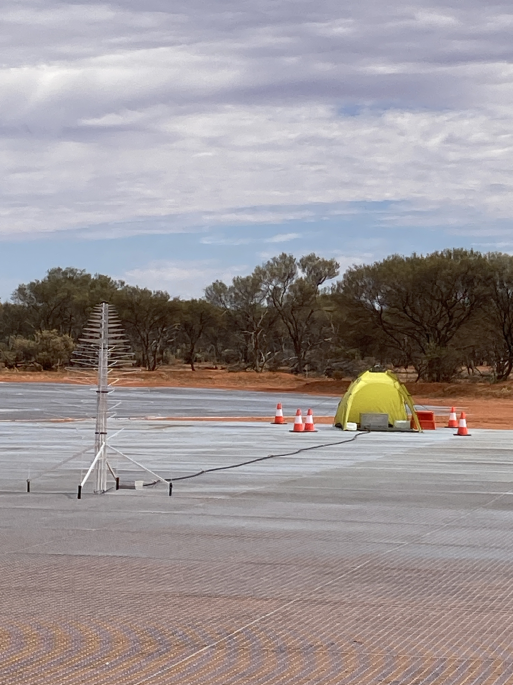
Our sky measurements were made with the GINAN receiver connected to a single SKALA4.1 antenna installed on a 40-m-diameter SKA-Low station ground mesh. The resulting observing system is shown schematically in Extended Data Fig. 1 and photographically in Fig. 1. Together, the new receiver and the accurately characterized antenna enable an accurate measurement of the radio sky in the SKA-Low band.

SKALA4.1 is a dual linearly polarized log-periodic antenna, designed for SKA-Low with the goal of realizing smooth frequency behaviour over the 50–350 MHz band⁴⁹. However, below 60 MHz, the antenna radiation efficiency has greater uncertainties associated with steeply rising resistive losses, exceeding 5%, in the metal of the antenna, mesh and ground. Therefore, only data in the range 60–350 MHz are used for accurate comparison with radio sky models. Extended Data Fig. 3 shows the antenna up close. There are ten solid and ten wire dipoles in each polarization. The feed lines for these 20 dipoles consist of a pair of rectangular tubes, which conduct the radiation received in that polarization to the vertex. The antenna is designed for 50-Ω single-ended feeding.

Sky measurements were made with the antenna placed at the centre of mesh S16-4 at the southern extremity of the SKA-Low telescope, within Inyarrimanha Ilgari Bundara, the CSIRO Murchison Radio-astronomy Observatory in Australia. The specific location was latitude −27.05934°, longitude 116.479561° and height 320.0 m. The quoted height is that of the ground mesh in geodetic coordinates with respect to the reference ellipsoid in the International Terrestrial Reference System frame. This mesh was one in a tight cluster of six meshes that were unpopulated at the time of our measurement. Each mesh will eventually host 256 SKALA4.1 antennas to form one SKA-Low station.

The mesh was constructed from 4-mm-diameter wire welded together on a 50 mm × 50 mm square grid. This yielded a ground plane conductivity of 0.2 MS m⁻¹, lower than might be expected for a metallic structure due to galvanization of the mesh. The mesh was made from hot-dipped galvanized steel, which is steel with a coating of zinc in the form of layered zinc–steel alloy that lowers the conductivity substantially⁶⁷.

Simulations were made to examine the effect of ground pickup from below and beyond the mesh. Antenna patterns derived from an electromagnetic simulation using soil below the mesh of relative permittivity ϵ_r = 4 and conductivity σ_soil = 0.7 mS m⁻¹ showed no difference to the patterns used in the current work that ignored soil below the mesh. This indicates that insufficient currents or side-lobe power reaches the lossy ground in the first place to be able to dissipate there.

The antenna was pointed at the zenith, and its polarizations were oriented in the E–W and N–S directions. Our measurements were made with the E–W-oriented dipole arms with the unused N–S-oriented arms terminated in 50 Ω, which is close to the antenna impedance over most of the band. Supplementary Fig. 1 shows the principal half-power beamwidths versus frequency for the selected E–W-oriented linear polarization state, as simulated in the H plane (N–S) and E plane (E–W). As expected for E–W-oriented dipoles, the beamwidth was larger in the N–S H plane. The mean half-power beamwidth over the operational frequency range was 64° in the E–W plane and 82° in the N–S plane.

Small glitches disrupt the beamwidth smoothness at different frequencies. These are due to spurious radiation of secondary dipole harmonics and have been confirmed in anechoic chamber measurements of the antenna⁶⁸. The antenna patterns from the electromagnetic simulations shown here, which capture the sharp features, were directly used to derive our offset and scale factors for correcting GSM2016. Hence, this anomaly in antenna behaviour has been accounted for in our analysis.

Supplementary Fig. 2 shows antenna pattern cuts at 145 MHz for three fixed azimuth angles. There was a wider beam with larger side lobes at azimuth 0° compared with azimuth 90°. The response to the horizon went to zero at all azimuths. Supplementary Fig. 3 shows beam footprints on the sky at the 3-dB and 10-dB gain levels.

The SKALA4.1 antenna usually incorporates a low-noise amplifier (LNA) at the apex of each of its two polarizations. We replaced these with modified end caps so that we could use the antenna with the external GINAN receiver that incorporates its own LNA. The feed lines corresponding to the unused N–S polarization dipoles were terminated at the apex in a 50-Ω load enclosed in an end cap (Supplementary Fig. 4a). A 3.1-m low-loss FSJ1 HELIAX coaxial cable was passed through from the base to the apex of one of the feed lines corresponding to the E–W polarization used for measurements. At the apex, the coaxial cable was connected to an SMB coaxial RF connector on a small printed circuit board that connects the cable ground with that of the feed leg hosting the cable and connects the cable core via a short 50-Ω transmission line to the opposite feed line. Supplementary Fig. 4b shows the resulting connectorized end cap. Both the 50-Ω load end cap and the connectorized end cap are modifications of the original SKALA4.1 LNA cap assembly shown in Supplementary Fig. 4c.

The GINAN receiver was split between a pair of enclosures: a small unit close to the antenna base (Extended Data Fig. 3) to which the 3.1-m coaxial cable connects and a larger unit placed 19 m away in a small tent at the edge of the ground mesh (Fig. 1). The smaller and larger units are connected by a 19-m low-loss LDF4-50A HELIAX coaxial cable to receive the RF signal from the antenna. They are also connected by a second lower-quality coaxial cable through which control pulses are sent from the larger box to an RF switch in the smaller box. These pulses control whether the receiver is connected to a particular calibration load or the antenna.

Wideband radiometric calibration

As stated in section ‘GINAN receiver with advanced architecture’, in each calibration cycle, the switch cycles through all five RF loads and the antenna. Measurements are made in each of these six switch positions with both the VNA and spectrometer to derive receiver and antenna calibrations. The five RF loads are precision short, precision open, precision 50 Ω, a network with complex impedance and a calibrated noise source that is temperature-compensated.

Based on measurements within each calibration cycle, we first solved for the error terms in the VNA using measurements of the reflection coefficients for standard precision terminations. With those corrections applied, the complex impedance of the antenna and receiver, the complex load and the internal calibrated noise source were measured. Using these complex impedances and the measurements made by the spectrometer of the power spectra from the set of internal terminations, which include a 50-Ω termination with temperature probe attached and the temperature-compensated excess noise source, we derived a joint solution for the noise waves and band-pass. The noise waves are described by four real-valued parameters. The band-pass describes the passband shape and also provides a scaling of the spectrometer counts to the antenna temperature in kelvins. The noise waves and scale are referenced to the input terminals of the GINAN receiver.

The GINAN receiver performs this full internal calibration in cycles with a cadence of 4 min. This time was set based on laboratory studies of the stability of the electronics. All calibrations, including the four-parameter model for the noise waves, were derived per channel and solved for independently in each frequency channel and in each calibration cycle. The VNA provided 2,001 independent measurements over 30–350 MHz. The spectrometer provided 4,001 measurements with a 100-kHz resolution bandwidth over 30–350 MHz. Impedance computations at the spectral measurement points of the network analyser were interpolated to the channelization frequencies of the spectrometer. The calibration was applied to the spectrometer measurements made with the switch connected to the antenna plus its feed cable to derive calibrated sky spectra for each calibration cycle. These calibrated sky spectra are for the antenna temperature at the terminals of the GINAN receiver on an absolute noise-temperature scale in kelvins, corrected for receiver noise waves, receiver band-pass and for any impedance mismatch between the antenna and receiver at the terminals of the GINAN receiver. The calibrated spectra have the native resolution and channel spacing of the spectrometer.

Calibrating the reflections and receiver noise waves

The switch acts as the main calibration reference plane, and calibration is performed on a per-cycle basis. Each cycle includes measurements of all switch positions using both the VNA and the spectrometer. The architecture of the GINAN receiver allows for direct VNA measurement of the complex reflection coefficient of the antenna plus feed cable relative to the receiver. The VNA also directly measures the complex reflection coefficients of the noise source, 50-Ω load and complex RF load relative to the receiver. We adopted the simplified model of the receiver noise waves shown in Supplementary Fig. 5. The measured complex reflection coefficients along with the noise wave parameters provide accurate estimates of the receiver noise in each of the spectrometer measurements made with the switch connected to one of the RF loads or antenna. Additionally, the impedance of the aggregate antenna and cable and the impedance of the receiver were determined separately relative to the 50-Ω reference, which allowed us to determine the power transfer function for the radiometer.

With the switch connected to one of the six terminations, the complex reflection coefficient Γ_1t of the termination impedance relative to the receiver impedance is given by

where Γ_m is the reflection coefficient as measured by the VNA S₂₁ measurement with ports labelled as per Extended Data Fig. 1. ϵ₀₀ and g₂₁ are the leakage and gain, respectively, within the receiver architecture between the two ports of the VNA. We solved for the leakage and gain separately in each VNA frequency channel and in each calibration cycle using VNA measurements of the reflection coefficients when the switch was connected to the precision open and short terminations.

Additionally, using the VNA measurement of the complex reflection coefficient in each switch setting, the complex reflection coefficient Γ_2t of that termination relative to the 50-Ω reference is given by

where the VNA calibration terms a, b and c are solved for using VNA measurements of reflection coefficients Γ_mo, Γ_ms and Γ_ml that were made with the switch connected to the precision open, precision short and precision 50-Ω terminations, respectively. These VNA calibration terms are related to the leakage, gain and another source match term ϵ₁₁ by the relations: a = g₂₁ − ϵ₀₀ϵ₁₁, b = ϵ₀₀ and c = −ϵ₁₁.

The complex impedance of the GINAN receiver relative to the Z₀ = 50-Ω reference is given by

Therefore, the power transfer to the GINAN receiver from a termination with noise temperature T_t and impedance Z_t is \({T}_{{\rm{t}}}(1-{\zeta }_{{\rm{t}}}{\zeta }_{{\rm{t}}}^{* })\), where \({\zeta }_{{\rm{t}}}=({Z}_{{\rm{r}}}-{Z}_{{\rm{t}}}^{* })/({Z}_{{\rm{r}}}+{Z}_{{\rm{t}}}^{* })\), and the superscript * denotes complex conjugation.

The spectrometer measurement contains the additive sum of (1) this noise temperature from the termination transferred to the GINAN receiver \({T}_{{\rm{t}}}(1-{\zeta }_{{\rm{t}}}{\zeta }_{{\rm{t}}}^{* })\), and (2) receiver noise generated in the GINAN receiver, which includes emission from the LNA and other active devices in the RF signal path, Nyquist–Johnson (thermal) noise from the passive components such as couplers, attenuators, cables and connectors, and the additive quantization noise in the analogue-to-digital converters. As shown in Supplementary Fig. 5, the total receiver noise is modelled as a pair of noise voltage waves⁶⁴ relative to the switch plane: N₁ travelling upstream towards the terminations or antenna and N₂ travelling downstream in the direction of the RF signal flow. Relative to the switch plane, the total receiver noise voltage arriving at the spectrometer is

where Γ_1t is the complex reflection coefficient of the termination with respect to the receiver.

Thus, the total noise power P_sys received by the spectrometer in units of spectrometer counts is

where T_sys is the total noise temperature received by the spectrometer in kelvins, B_p is the GINAN receiver band-pass function representing the spectral gain of the receiver that converts system temperature to spectrometer counts and ℜ[⋅] is the real part. B_p has units of spectrometer counts per kelvin noise temperature.

Calibrating for additive receiver noise and the band-pass function requires solving for the five calibration terms \({N}_{1}{N}_{1}^{* }\), \({N}_{2}{N}_{2}^{* }\), \(\Re [{N}_{1}{N}_{2}^{* }]\), \(\Im [{N}_{1}{N}_{2}^{* }]\) and B_p, where ℑ[⋅] is the imaginary part. Spectrometer measurements of the total power with the switch connected to the precision open, precision short, network with complex impedance, precision 50 Ω, and calibrated noise source provide a set of five linear equations with these five calibration terms as variables. We used a chi-squared solver on this set to simultaneously estimate the five calibration terms. In situ temperature logger recordings of the precision 50-Ω termination and a laboratory calibration of the noise temperature of the temperature-compensated noise source (section ‘Calibrating the temperature scale’) were used in the solution. The calibration terms were derived independently for each calibration cycle and for each spectrometer frequency channel. The network with complex impedance, which is used as one of the calibration RF loads at the switch, was selected, so that solutions for all five GINAN receiver calibration terms were possible without singularities over the entire operating frequency range. This required the network to be an inductance.

Finally, the calibrated noise temperature T_t available at the end of the antenna feed cable (at the switch input) was evaluated by inverting equation (8) for all spectra where the switch was connected to the antenna. Substituting in noise wave terms, the band-pass, the complex reflection coefficient of the antenna (including its cable) relative to the GINAN receiver and the power transfer function \((1-{\zeta }_{{\rm{t}}}{\zeta }_{{\rm{t}}}^{* })\) yielded the antenna temperature in kelvins from any given spectrometer noise power spectrum P_sys. A unique aspect of the GINAN receiver is that it can evaluate and apply all of these calibration terms every 4 min, in situ while connected to the antenna.

Calibrating the temperature scale

The absolute calibration scale is set by the spectral noise powers from the internal 50-Ω termination, whose temperature is monitored during the observations, and the temperature-compensated internal noise source. Laboratory calibration accurately determined the noise temperature of the internal noise source and was used to model for any offset between the noise temperature of the internal 50-Ω termination and its physical temperature, as given by a temperature probe affixed to that termination.

In the laboratory, an external 50-Ω termination with a temperature probe affixed was placed in an insulated water bath and connected to the input terminals of the GINAN receiver in place of the antenna. With the GINAN receiver cycling through its calibration and acquisition of spectra process, the bath was first maintained at a stable low temperature with ice, which was replaced with boiling water that was allowed to cool slowly to ambient temperature over hours. With the noise temperature of the internal noise source assigned a value corresponding to its manufacturer’s datasheet, all receiver calibrations were derived and applied. The calibration includes corrections for the power transfer from the external 50-Ω termination to the GINAN receiver and for the receiver noise waves that are conditioned by the voltage reflection coefficient of this external 50-Ω termination impedance relative to that of the GINAN receiver. The estimated noise temperature of the external 50-Ω termination that was immersed in the bath was then compared with the physical temperature reading of the probe affixed to that termination. The probe temperature varied from close to 0 °C to somewhat above 70 °C, and linear fits to the noise temperature versus probe temperature yielded a slope and offset at each frequency bin.

The factor by which the slope of the fit departed from unity is the fractional error in the value assigned to the noise source. The offset in the intercept from the origin is the difference between the noise temperature of the internal 50-Ω termination and the reading provided by the attached temperature probe. Using the slopes of the linear fits over frequency, we modelled the profile of the noise source, as shown in Supplementary Fig. 6. Using the offsets from the origin in the linear fits, we modelled the noise temperature of the internal termination in terms of the temperature probes affixed to the termination and within the GINAN receiver enclosure.

Adopting this laboratory calibration for the noise source and internal termination and, hence, for the temperature scale, the slope and offset in the linear fits to the noise temperature versus probe temperature are shown in Supplementary Fig. 7 for the 60–350-MHz band. The fits were made at the native spectrometer channel spacing of 80 kHz. The slopes and offset values are also displayed after Hanning smoothing with a 10-MHz window. For measurements made with these bandwidths, the uncertainty of calibration has an r.m.s. value of 0.5% in scale and 1.5 K in offset.

Calibrating the antenna cable

The terminals of the SKALA4.1 antenna are located at its vertex. A customized end cap (Supplementary Fig. 4b) allows the antenna terminals to be connected by a low-loss coaxial cable to the RF switch of the GINAN receiver, which is in a small enclosure at the base of the antenna (Extended Data Fig. 3). As the switch serves as the calibration reference plane, we needed to determine the cable characteristics and correct the data for the multiplicative cable transfer function and additive thermal noise. The 3.1-m cable was positioned inside the antenna strut with its top end disconnected at the antenna vertex, and a temperature probe was added midway down its length. A precision 50-Ω termination was connected at the top end of the cable in place of the antenna, and the GINAN radiometer was cycled through its measurements and calibration steps. This was repeated with the termination replaced by a precision open circuit and then a precision short. The cable was at ambient temperature during this calibration measurement. The GINAN receiver calibration process provided accurate measurements of the impedance and thermal emission spectrum of the cable with these terminations. These measured quantities are related to the cable attenuation, physical temperature, velocity factor and characteristic impedance, and hence, they were used to solve for these properties.

The noise-temperature spectrum emerging from the cable can be considered to be composed of three parts: (1) thermal emission generated in the cable resistance and directed downstream towards the receiver; (2) thermal emission generated in the cable resistance that is directed upstream away from the receiver and then reflected back by the impedance mismatch between the cable and the 50-Ω open or short termination; and (3) interference between the coherent parts of the random voltages corresponding to these two noise components. These receiver noise components can be modelled as noise waves⁶⁴. We derived the cable properties by fitting the models for the cable impedance and cable emission spectra to the measurements made by the VNA and the spectrometer. Supplementary Fig. 8 shows the solutions derived from these measurements for cable attenuation, velocity factor and complex cable characteristic impedance.

Using these solutions for the cable properties along with measurements of the physical temperature of the cable and the 50-Ω termination at the cable end that were made using temperature probes, we predicted the noise-temperature spectra at the GINAN receiver terminals owing to the thermal emission of the cable. These predictions are compared with measurements in Supplementary Fig. 9. For a reasonably well matched antenna, we expect the errors in our modelling of the characteristics of the 3.1-m cable, along with in situ measurements of its temperature, to enable a correction for cable additive thermal emission with an r.m.s. error of less than 1 K. The cable attenuation was less than 10%, and the accuracy of the measurement of the cable attenuation by the VNA embedded in the receiver was about 1%. Therefore, the error in cable attenuation resulted in a scale calibration error of less than about 0.1%.

Note that the GINAN receiver was designed to be connected directly to the terminals of an antenna. Not using a cable between the antenna and the receiver results in lower loss and a smoother band-pass. This simplifies the calibration required to detect the very weak signals that GINAN targets, like the all-sky signal of the redshifted 21-cm line during cosmic dawn. There is no need to additionally calibrate and model the attenuation and emission from the antenna feed cable when the GINAN receiver is directly connected to the terminals of an antenna. Direct connection removes one of the few remaining manual calibration steps in the field (attaching calibration loads to the antenna end of the feed cable), removes the need to measure the temperature of the feed cable and reduces measurement uncertainty.

For the absolute temperature measurement of the radio sky that we have made using the GINAN receiver and SKALA4.1 antenna, the cable is inevitable and, hence, needs to be accounted for. The noise waves that our derived model predicts for the cable used to connect the SKALA4.1 antenna to the GINAN receiver are shown in Supplementary Fig. 10. The calibrated noise temperature available at the base of the antenna cable, following the calibration steps discussed in section ‘Calibrating the reflections and receiver noise waves’, was corrected for these noise waves that our model predicts for the cable and for the measured attenuation in the antenna cable. Additionally, a correction was made for the power transfer from the SKALA4.1 antenna to the antenna cable, based on derivations of the impedances of the antenna at its vertex and of the GINAN receiver as referenced at the top end of the antenna cable at the antenna vertex. This yielded calibrated antenna-temperature spectra for each calibration cycle.

Calibration validation

The data measured by the spectrometer were corrected so that we could derive accurate radio-sky brightness spectra in the form of antenna-temperature spectra. The various stages of correction are illustrated in Supplementary Fig. 11. Internal radiometer corrections were applied first: the multiplicative band-pass of the receiver system was calibrated, and then the spectrum was corrected for receiver additive noise. Next, corrections were made for the attenuation and additive thermal noise caused by the cable connecting the antenna to the receiver. Then the transfer function through the antenna to the cable (including the antenna–receiver impedance mismatch) was calibrated. Last, a correction was made for antenna radiation efficiency, which includes the resistive loss in the antenna and 40-m ground mesh. Each calibration step resulted in smoother measured spectra that were closer to the GSM2016-predicted antenna temperature in both amplitude and spectral index.

The precision of the end-to-end calibration algorithm and implementation was tested by using an antenna emulator. This consisted of a poorly matched RLC circuit with a real impedance of 25 Ω. Once the calibration was applied, this produced a flat spectral response at 292 K corresponding to ambient temperature. The standard deviation of the spectrum over the entire band was approximately 400 mK. This gave us confidence that the calibration scheme removed both the multiplicative and additive errors while also correctly scaling the result. Additionally, we verified the power transfer (impedance mismatch) correction made by the GINAN receiver by extracting the complex impedance of the antenna from the receiver calibration parameters. This agreed well with the predictions of an electromagnetic simulation of the antenna and ground mesh.

Systematic uncertainties

The total systematic uncertainty in our measurement of the sky radio brightness is the quadrature sum of errors arising from the absolute receiver calibration uncertainty, the antenna cable attenuation and emission uncertainties, the antenna pattern uncertainty, and the uncertainty arising from our use of a single linear polarization to measure the radio-sky brightness, which could be polarized.

Absolute calibration uncertainty

The absolute calibration of the GINAN receiver measurement was set by a laboratory calibration of the internal noise source, as described in section ‘Calibrating the temperature scale’. The dynamic self-calibration procedures used in the field measurements were all used in the laboratory calibration. This included calibrations for the band-pass profile and gain, receiver noise waves and impedance mismatches. The residuals of the linear fits to the calibrated noise temperature versus probe temperature in section ‘Calibrating the temperature scale’ demonstrate that the absolute calibration of the temperature scale has an uncertainty with an r.m.s. value of 0.5% in scale and 1.5 K in offset.

Cable attenuation and emission uncertainties

The 3.1-m cable connecting the antenna to the receiver attenuates the received signal and also adds its own thermal noise to the sky signal received. The measurement data were calibrated for the cable based on accurate laboratory measurements of the cable properties made using the GINAN receiver and in situ measurements of the impedance mismatches during signal propagation from the antenna via this cable to the receiver. These measurements and derived corrections are discussed in section ‘Calibrating the antenna cable’. The error in the cable thermal emission, which appears as an additive to be subtracted from the measurement data, was estimated to have an r.m.s. value of less than 1 K. The error in cable attenuation resulted in a scale calibration error of less than about 0.1%.

Antenna pattern uncertainty

The antenna pattern computed by the electromagnetic simulations was convolved with the model sky to give an expectation for the calibrated measurement. Errors in the electromagnetic simulation model for the pattern translate to errors in expectation for the measurement, given any global sky model. Consequently, comparisons between the measured and expected sky brightness yield erroneous corrections for the model sky. The errors in electromagnetic simulations are usually quantified by comparing the results of simulations made using different packages and methods. The isolated SKALA4.1 antenna on the ground plane was modelled⁴⁹ using FEKO and, separately, CST Studio Suite, MWS. The directivities at zenith and off zenith agreed well. Comparisons have also been made⁶⁹ for this antenna between FEKO and Galileo. Differences in the amplitude gain show that errors in individual patterns are not random over azimuth and elevation but systematic and, hence, would not be expected to diminish in the averaging over the pattern. Second, the error patterns are substantially different at different frequencies. Last, the magnitude of the error in the power pattern was less than 1%. It follows that the forward modelling of the global sky model brightness to the measurement could result in less than 1% error at individual frequencies, with uncorrelated errors across the band.

Uncertainty from use of a single linear polarization mode

We measured the radio-sky intensity using a single linear polarization mode; therefore, sky polarization is expected to manifest in a confusing spectral structure. Simulations⁷⁰ of the polarized radio sky and Faraday depth at long wavelengths show that r.m.s. values of the spectral confusion arising from measurements of the total intensity using single-polarization radiometers would be in the range 150 mK to 200 mK, with perhaps an extended tail up to 400 mK, when averaged over the wide beams of the broadband dipole-like antennas. Hence, errors in measurements of the radio-sky brightness in our observing band, made using a single polarization mode, are expected to have r.m.s. values of less than 0.4 K owing to the polarization of the brightness.

Total measurement uncertainty

Adding the above four sources of error in quadrature yields the r.m.s. values for the uncertainty in our measurement of the radio-sky brightness temperature. We display this versus frequency as the dotted line in Fig. 5. At 150 MHz, the r.m.s. value for the measurement uncertainty is 1.22%.

Uncertainty in the derived corrections to GSM2016

Any global sky model, including the GSM2016 for which we have derived corrections, could not only have errors in the form of a global offset and scale factor but could, in addition, have systematic errors that vary over the sky. Such errors would manifest in residual differences between the measurements and predictions for these measurements that are made after correcting the global sky model with the best-fitting offset and scale factor. The dashed-dotted line in Fig. 5 shows the r.m.s. value of the fractional difference between our measurements and our corrected GSM2016; at 150 MHz, this r.m.s. value is 1.33%. Such errors in sky maps would confuse the derivation of global offset and scale factor corrections.

Given the calibration accuracy of the GINAN receiver and the quality of modelling of the SKALA4.1 antenna, it is not surprising that the errors in our derived corrections to GSM2016 are dominated by errors in the images that were used to construct the sky model: errors that are not representable as global offsets and scale factors. Figure 5 shows how we added in quadrature these errors arising from such inaccuracies in GSM2016 (dashed-dotted line) to the r.m.s. values of uncertainty in our measurement of the radio-sky brightness temperature (dotted line) to get the total uncertainty in the corrected GSM2016 (solid line). At 150 MHz, the uncertainty in the corrected GSM2016 is 1.81%.